LTV

Invalidity of The

LTV Model

For Real Circuits

Kevin Aylward B.Sc.

www.kevinaylward.co.uk

Overview

It is shown that modelling real, physical oscillators with a Linear Time Variant (LTV) model is, in general, invalid. For example, the Hajimiri-Lee LTV phase noise theory. In particular:

A. Dimre shows that,

… The right-hand-side (RHS) of the differential equation (13) for the phase error is nonlinear. Thus, one can not use superposition to calculate the phase error due to several perturbations, i.e., one can not calculate the phase errors due to two perturbations separately and then sum them up to obtain the phase error due to the two perturbations applied at the same time.

and

1 A. Demi¹, with reference to the HL model, mathematically proves and states:

1.1 Is the orthogonal decomposition valid in general?

1.2 Even if it is not strictly valid, can it provide approximately correct results and intuition for practical oscillator designs?

1.3 We show that the answer to both questions is negative.

1.4 ...it can predict results off by as much as 50 dBc/Hz.

In the paper “ On the Validity of Orthogonally Decomposed Perturbations in Phase Noise Analysis”.

How is this shown without the somewhat obtuse, professional level mathematics of said paper?

Introduction

In principle, any system can initially be attempted to be explained by a Linear Time Variant (LTV) model in an attempt to reduce the complexity of an otherwise non-linear system. What matters though, is whether or not that mathematical abstract remodelling of a system can actually explain all of the key features of that real system which, in general, really does have non-linear components, independent of time.

It is a fact of linear, time invariant, system theory that such a system with many inputs can only produce output frequencies that are present at its input. So eyebrows may well be raised by the HL production, apparently from thin air, of an expression that contains the potential for such extra frequency components.

In a non-linear system it is not possible to calculate the output of a system signal with two frequency components simply by calculating the output due to each one, then adding the two outputs. Such an approach fails to include the effect of cross multiplication of the two input signals. For example, two signals applied to a circuit with some square law behaviour will contain sum and difference frequencies of the two signals.

It is, essentially, claimed in the HL-LTV theory that all major effects of such real non-linear systems may be alternatively explained by considering those components linear, but with their changes being due to time variance as dictated by an oscillator waveform. In such a way, the theory attempts to manifest the additional generated frequencies due to the simple properties of time variant systems for linear systems. It is shown here that such an alternative description of real components, fails.

LTV Model

The HL LTV model states that, given an input signal, the output phase can be calculated by:

ϕ 0 (t)= ∫ −∞ t I i (τ) Γ( ω 0 τ)dτ MathType@MTEF@5@5@+=feaagCart1ev2aaatCvAUfeBSjuyZL2yd9gzLbvyNv2CaerbuLwBLnhiov2DGi1BTfMBaeXatLxBI9gBaerbd9wDYLwzYfdmGievaebbnrfifHhDYfgasaacH8YjY=vipgYlh9vqqj=hEeeu0xXdbba9frFj0=OqFfea0dXdd9vqai=hGuQ8kuc9pgc9q8qqaq=dir=f0=yqaiVgFr0xfr=xfr=xb9adbaqaaeGaciGaaiaabeqaamaabaabaaGcbaGaeqy1dy2aaSbaaSqaaiaaicdaaeqaaOGaaiikaiaadshacaGGPaGaeyypa0Zaa8qCaeaacaWGjbWaaSbaaSqaaiaadMgaaeqaaOGaaiikaiabes8a0jaacMcaaSqaaiabgkHiTiabg6HiLcqaaiaadshaa0Gaey4kIipakiabfo5ahjaacIcacqaHjpWDdaWgaaWcbaGaaGimaaqabaGccqaHepaDcaGGPaGaamizaiabes8a0baa@5091@

Where Γ( ω 0 τ) MathType@MTEF@5@5@+=feaagCart1ev2aaatCvAUfeBSjuyZL2yd9gzLbvyNv2CaerbuLwBLnhiov2DGi1BTfMBaeXatLxBI9gBaerbd9wDYLwzYfdmGievaebbnrfifHhDYfgasaacH8YjY=vipgYlh9vqqj=hEeeu0xXdbba9frFj0=OqFfea0dXdd9vqai=hGuQ8kuc9pgc9q8qqaq=dir=f0=yqaiVgFr0xfr=xfr=xb9adbaqaaeGaciGaaiaabeqaamaabaabaaGcbaGaeu4KdCKaaiikaiabeM8a3naaBaaaleaacaaIWaaabeaakiabes8a0jaacMcaaaa@3CF9@ is what is named as the Impulse Sensitivity Function, ISF.

By construction, this method requires that Γ( ω 0 τ) MathType@MTEF@5@5@+=feaagCart1ev2aaatCvAUfeBSjuyZL2yd9gzLbvyNv2CaerbuLwBLnhiov2DGi1BTfMBaeXatLxBI9gBaerbd9wDYLwzYfdmGievaebbnrfifHhDYfgasaacH8YjY=vipgYlh9vqqj=hEeeu0xXdbba9frFj0=OqFfea0dXdd9vqai=hGuQ8kuc9pgc9q8qqaq=dir=f0=yqaiVgFr0xfr=xfr=xb9adbaqaaeGaciGaaiaabeqaamaabaabaaGcbaGaeu4KdCKaaiikaiabeM8a3naaBaaaleaacaaIWaaabeaakiabes8a0jaacMcaaaa@3CF9@ be linear, periodic and independent of the input signal. If I i (τ) MathType@MTEF@5@5@+=feaagCart1ev2aaatCvAUfeBSjuyZL2yd9gzLbvyNv2CaerbuLwBLnhiov2DGi1BTfMBaeXatLxBI9gBaerbd9wDYLwzYfdmGievaebbnrfifHhDYfgasaacH8YjY=vipgYlh9vqqj=hEeeu0xXdbba9frFj0=OqFfea0dXdd9vqai=hGuQ8kuc9pgc9q8qqaq=dir=f0=yqaiVgFr0xfr=xfr=xb9adbaqaaeGaciGaaiaabeqaamaabaabaaGcbaGaamysamaaBaaaleaacaWGPbaabeaakiaacIcacqaHepaDcaGGPaaaaa@3AC6@ is the sum of two independent noise frequencies, the output phase cannot contain any sum and difference frequencies of those inputs by design. The procedure of the HL LTV approach is to calculate for each noise source the resulting phase noise and combine them by superposition. This procedure thus ignores the mixed product interaction between noise frequency components. However, in real, typical circuits it can be shown that such mixed products do exist. The LTV model approach is therefore not physically valid. It is also mathematically contradictory.

Phase Modulator

The following analyses the effect of noise signals on the phase of another signal in a typical circuit.

Fig. 1

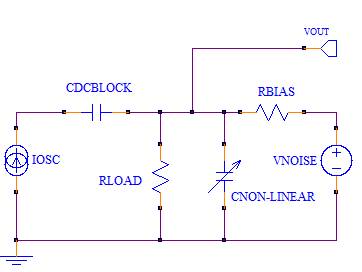
Fig. 1 is a very typical topology, representative of many real circuit applications, not necessarily restricted to oscillators, but most oscillators can be topologically resolved to the analysis of this topology. For the purposes of this discussion, it is assumed that the IOSC current is large, and at a much higher frequency than that produced by VNOISE. VNOISE is assumed to be very small and of low frequency, typically down to DC. CNON_LINEAR is a non linear capacitance, not necessarily a purpose variactor, but illustrates that any real, physical circuit always contains non linear capacitance. However, it should also be noted that it could be the resistor that varies with the capacitor constant. All that matters is that there is a time constant that varies with voltage. In the absence of any noise voltage, VOUT will thus be an output reflecting the IOSC signal. Adding in a very small noise voltage to the capacitor will have some small effect on the amplitude of VOUT, but for the purposes of calculating the effect of this noise on the phase of VOUT, can be ignored. VOUT can therefore be expressed as:

Vout= V o sin( ω 0 t+Φ(t)) MathType@MTEF@5@5@+=feaagCart1ev2aqatCvAUfeBSjuyZL2yd9gzLbvyNv2CaerbuLwBLnhiov2DGi1BTfMBaeXatLxBI9gBaerbd9wDYLwzYfdmGievaebbnrfifHhDYfgasaacH8YjY=vipgYlh9vqqj=hEeeu0xXdbba9frFj0=OqFfea0dXdd9vqai=hGuQ8kuc9pgc9q8qqaq=dir=f0=yqaiVgFr0xfr=xfr=xb9adbaqaaeGaciGaaiaabeqaamaabaabaaGcbaGaamOvaiaad+gacaWG1bGaamiDaiabg2da9iaadAfadaWgaaWcbaGaam4BaaqabaGccaWGZbGaamyAaiaad6gacaGGOaGaeqyYdC3aaSbaaSqaaiaaicdaaeqaaOGaamiDaiabgUcaRiabfA6agjaacIcacaWG0bGaaiykaiaacMcaaaa@491A@

With the phase, Φ(t) MathType@MTEF@5@5@+=feaagCart1ev2aqatCvAUfeBSjuyZL2yd9gzLbvyNv2CaerbuLwBLnhiov2DGi1BTfMBaeXatLxBI9gBaerbd9wDYLwzYfdmGievaebbnrfifHhDYfgasaacH8YjY=vipgYlh9vqqj=hEeeu0xXdbba9frFj0=OqFfea0dXdd9vqai=hGuQ8kuc9pgc9q8qqaq=dir=f0=yqaiVgFr0xfr=xfr=xb9adbaqaaeGaciGaaiaabeqaamaabaabaaGcbaGaeuOPdyKaaiikaiaadshacaGGPaaaaa@3983@ , of the IOSC signal subsequently derived to be:

Φ(t)= tan −1 ( ω 0 CR) MathType@MTEF@5@5@+=feaagCart1ev2aaatCvAUfeBSjuyZL2yd9gzLbvyNv2CaerbuLwBLnhiov2DGi1BTfMBaeXatLxBI9gBaerbd9wDYLwzYfdmGievaebbnrfifHhDYfgasaacH8YjY=vipgYlh9vqqj=hEeeu0xXdbba9frFj0=OqFfea0dXdd9vqai=hGuQ8kuc9pgc9q8qqaq=dir=f0=yqaiVgFr0xfr=xfr=xb9adbaqaaeGaciGaaiaabeqaamaabaabaaGcbaGaeuOPdyKaaiikaiaadshacaGGPaGaeyypa0JaciiDaiaacggacaGGUbWaaWbaaSqabeaacqGHsislcaaIXaaaaOGaaiikaiabeM8a3naaBaaaleaacaaIWaaabeaakiaadoeacaWGsbGaaiykaaaa@44ED@

Where the R and C in relation to Fig. 1 is left to the reader to figure out!

Typically, the voltage variance of C may contain several power orders of voltage, but even if C had only a linear term, the atan() function ensures that Φ(t) MathType@MTEF@5@5@+=feaagCart1ev2aqatCvAUfeBSjuyZL2yd9gzLbvyNv2CaerbuLwBLnhiov2DGi1BTfMBaeXatLxBI9gBaerbd9wDYLwzYfdmGievaebbnrfifHhDYfgasaacH8YjY=vipgYlh9vqqj=hEeeu0xXdbba9frFj0=OqFfea0dXdd9vqai=hGuQ8kuc9pgc9q8qqaq=dir=f0=yqaiVgFr0xfr=xfr=xb9adbaqaaeGaciGaaiaabeqaamaabaabaaGcbaGaeuOPdyKaaiikaiaadshacaGGPaaaaa@3983@ is a non-linear function of the applied noise voltage. For example, a low order approximation might be:

C= C 0 (1+ k v1 v n + k v2 v n 2 ) MathType@MTEF@5@5@+=feaagCart1ev2aaatCvAUfeBSjuyZL2yd9gzLbvyNv2CaerbuLwBLnhiov2DGi1BTfMBaeXatLxBI9gBaerbd9wDYLwzYfdmGievaebbnrfifHhDYfgasaacH8YjY=vipgYlh9vqqj=hEeeu0xXdbba9frFj0=OqFfea0dXdd9vqai=hGuQ8kuc9pgc9q8qqaq=dir=f0=yqaiVgFr0xfr=xfr=xb9adbaqaaeGaciGaaiaabeqaamaabaabaaGcbaGaam4qaiabg2da9iaadoeadaWgaaWcbaGaaGimaaqabaGccaGGOaGaaGymaiabgUcaRiaadUgadaWgaaWcbaGaamODaiaaigdaaeqaaOGaamODamaaBaaaleaacaWGUbaabeaakiabgUcaRiaadUgadaWgaaWcbaGaamODaiaaikdaaeqaaOGaamODamaaBaaaleaacaWGUbaabeaakmaaCaaaleqabaGaaGOmaaaakiaacMcaaaa@4808@

tan −1 (x)~x− x 3 3 MathType@MTEF@5@5@+=feaagCart1ev2aaatCvAUfeBSjuyZL2yd9gzLbvyNv2CaerbuLwBLnhiov2DGi1BTfMBaeXatLxBI9gBaerbd9wDYLwzYfdmGievaebbnrfifHhDYfgasaacH8YjY=vipgYlh9vqqj=hEeeu0xXdbba9frFj0=OqFfea0dXdd9vqai=hGuQ8kuc9pgc9q8qqaq=dir=f0=yqaiVgFr0xfr=xfr=xb9adbaqaaeGaciGaaiaabeqaamaabaabaaGcbaGaciiDaiaacggacaGGUbWaaWbaaSqabeaacqGHsislcaaIXaaaaOGaaiikaiaadIhacaGGPaGaaiOFaiaadIhacqGHsisldaWcaaqaaiaadIhadaahaaWcbeqaaiaaiodaaaaakeaacaaIZaaaaaaa@4266@

Φ(t)= ω 0 R C 0 (1+ k v1 v n + k v2 v n 2 )− ω 0 3 R 3 C 0 3 3 (1+ k v1 v n + k v2 v n 2 ) 3 MathType@MTEF@5@5@+=feaagCart1ev2aaatCvAUfeBSjuyZL2yd9gzLbvyNv2CaerbuLwBLnhiov2DGi1BTfMBaeXatLxBI9gBaerbd9wDYLwzYfdmGievaebbnrfifHhDYfgasaacH8YjY=vipgYlh9vqqj=hEeeu0xXdbba9frFj0=OqFfea0dXdd9vqai=hGuQ8kuc9pgc9q8qqaq=dir=f0=yqaiVgFr0xfr=xfr=xb9adbaqaaeGaciGaaiaabeqaamaabaabaaGcbaGaeuOPdyKaaiikaiaadshacaGGPaGaeyypa0JaeqyYdC3aaSbaaSqaaiaaicdaaeqaaOGaamOuaiaadoeadaWgaaWcbaGaaGimaaqabaGccaGGOaGaaGymaiabgUcaRiaadUgadaWgaaWcbaGaamODaiaaigdaaeqaaOGaamODamaaBaaaleaacaWGUbaabeaakiabgUcaRiaadUgadaWgaaWcbaGaamODaiaaikdaaeqaaOGaamODamaaBaaaleaacaWGUbaabeaakmaaCaaaleqabaGaaGOmaaaakiaacMcacqGHsisldaWcaaqaaiabeM8a3naaBaaaleaacaaIWaaabeaakmaaCaaaleqabaGaaG4maaaakiaadkfadaahaaWcbeqaaiaaiodaaaGccaWGdbWaaSbaaSqaaiaaicdaaeqaaOWaaWbaaSqabeaacaaIZaaaaaGcbaGaaG4maaaacaGGOaGaaGymaiabgUcaRiaadUgadaWgaaWcbaGaamODaiaaigdaaeqaaOGaamODamaaBaaaleaacaWGUbaabeaakiabgUcaRiaadUgadaWgaaWcbaGaamODaiaaikdaaeqaaOGaamODamaaBaaaleaacaWGUbaabeaakmaaCaaaleqabaGaaGOmaaaakiaacMcadaahaaWcbeqaaiaaiodaaaaaaa@6838@

For a dominant square law capacitance at lower values of ω 0 R C 0 MathType@MTEF@5@5@+=feaagCart1ev2aaatCvAUfeBSjuyZL2yd9gzLbvyNv2CaerbuLwBLnhiov2DGi1BTfMBaeXatLxBI9gBaerbd9wDYLwzYfdmGievaebbnrfifHhDYfgasaacH8YjY=vipgYlh9vqqj=hEeeu0xXdbba9frFj0=OqFfea0dXdd9vqai=hGuQ8kuc9pgc9q8qqaq=dir=f0=yqaiVgFr0xfr=xfr=xb9adbaqaaeGaciGaaiaabeqaamaabaabaaGcbaGaeqyYdC3aaSbaaSqaaiaaicdaaeqaaOGaamOuaiaadoeadaWgaaWcbaGaaGimaaqabaaaaa@3AF8@ :

Φ(t)= ω 0 R C 0 (1+ k v2 v n 2 ) MathType@MTEF@5@5@+=feaagCart1ev2aaatCvAUfeBSjuyZL2yd9gzLbvyNv2CaerbuLwBLnhiov2DGi1BTfMBaeXatLxBI9gBaerbd9wDYLwzYfdmGievaebbnrfifHhDYfgasaacH8YjY=vipgYlh9vqqj=hEeeu0xXdbba9frFj0=OqFfea0dXdd9vqai=hGuQ8kuc9pgc9q8qqaq=dir=f0=yqaiVgFr0xfr=xfr=xb9adbaqaaeGaciGaaiaabeqaamaabaabaaGcbaGaeuOPdyKaaiikaiaadshacaGGPaGaeyypa0JaeqyYdC3aaSbaaSqaaiaaicdaaeqaaOGaamOuaiaadoeadaWgaaWcbaGaaGimaaqabaGccaGGOaGaaGymaiabgUcaRiaadUgadaWgaaWcbaGaamODaiaaikdaaeqaaOGaamODamaaBaaaleaacaWGUbaabeaakmaaCaaaleqabaGaaGOmaaaakiaacMcaaaa@48BE@

For the case of the noise voltage being the sum of two frequencies, and neglecting the constant term as irrelevant for the purposes of phase noise.

Φ(t)= ω 0 R C 0 k v2 ( v n1 + v n2 ) 2 MathType@MTEF@5@5@+=feaagCart1ev2aaatCvAUfeBSjuyZL2yd9gzLbvyNv2CaerbuLwBLnhiov2DGi1BTfMBaeXatLxBI9gBaerbd9wDYLwzYfdmGievaebbnrfifHhDYfgasaacH8YjY=vipgYlh9vqqj=hEeeu0xXdbba9frFj0=OqFfea0dXdd9vqai=hGuQ8kuc9pgc9q8qqaq=dir=f0=yqaiVgFr0xfr=xfr=xb9adbaqaaeGaciGaaiaabeqaamaabaabaaGcbaGaeuOPdyKaaiikaiaadshacaGGPaGaeyypa0JaeqyYdC3aaSbaaSqaaiaaicdaaeqaaOGaamOuaiaadoeadaWgaaWcbaGaaGimaaqabaGccaWGRbWaaSbaaSqaaiaadAhacaaIYaaabeaakiaacIcacaWG2bWaaSbaaSqaaiaad6gacaaIXaaabeaakiabgUcaRiaadAhadaWgaaWcbaGaamOBaiaaikdaaeqaaOGaaiykamaaCaaaleqabaGaaGOmaaaaaaa@4B94@

Hence, for sinusoidal noise voltages

Φ(t)= ω 0 R C 0 k v2 ( v n1pk sin ω 1 t+ v n2pk sin ω 2 t) 2 MathType@MTEF@5@5@+=feaagCart1ev2aaatCvAUfeBSjuyZL2yd9gzLbvyNv2CaerbuLwBLnhiov2DGi1BTfMBaeXatLxBI9gBaerbd9wDYLwzYfdmGievaebbnrfifHhDYfgasaacH8YjY=vipgYlh9vqqj=hEeeu0xXdbba9frFj0=OqFfea0dXdd9vqai=hGuQ8kuc9pgc9q8qqaq=dir=f0=yqaiVgFr0xfr=xfr=xb9adbaqaaeGaciGaaiaabeqaamaabaabaaGcbaGaeuOPdyKaaiikaiaadshacaGGPaGaeyypa0JaeqyYdC3aaSbaaSqaaiaaicdaaeqaaOGaamOuaiaadoeadaWgaaWcbaGaaGimaaqabaGccaWGRbWaaSbaaSqaaiaadAhacaaIYaaabeaakiaacIcacaWG2bWaaSbaaSqaaiaad6gacaaIXaGaamiCaiaadUgaaeqaaOGaci4CaiaacMgacaGGUbGaeqyYdC3aaSbaaSqaaiaaigdaaeqaaOGaamiDaiabgUcaRiaadAhadaWgaaWcbaGaamOBaiaaikdacaWGWbGaam4AaaqabaGcciGGZbGaaiyAaiaac6gacqaHjpWDdaWgaaWcbaGaaGOmaaqabaGccaWG0bGaaiykamaaCaaaleqabaGaaGOmaaaaaaa@5C7D@

Φ(t)= ω 0 R C 0 k v2 ( v n1pk 2 sin 2 ω 1 t+ v n1pk v n2pk sin ω 1 tsin ω 2 t+ v n2pk 2 sin 2 ω 2 t) MathType@MTEF@5@5@+=feaagCart1ev2aaatCvAUfeBSjuyZL2yd9gzLbvyNv2CaerbuLwBLnhiov2DGi1BTfMBaeXatLxBI9gBaerbd9wDYLwzYfdmGievaebbnrfifHhDYfgasaacH8YjY=vipgYlh9vqqj=hEeeu0xXdbba9frFj0=OqFfea0dXdd9vqai=hGuQ8kuc9pgc9q8qqaq=dir=f0=yqaiVgFr0xfr=xfr=xb9adbaqaaeGaciGaaiaabeqaamaabaabaaGcbaGaeuOPdyKaaiikaiaadshacaGGPaGaeyypa0JaeqyYdC3aaSbaaSqaaiaaicdaaeqaaOGaamOuaiaadoeadaWgaaWcbaGaaGimaaqabaGccaWGRbWaaSbaaSqaaiaadAhacaaIYaaabeaakiaacIcacaWG2bWaaSbaaSqaaiaad6gacaaIXaGaamiCaiaadUgaaeqaaOWaaWbaaSqabeaacaaIYaaaaOGaci4CaiaacMgacaGGUbWaaWbaaSqabeaacaaIYaaaaOGaeqyYdC3aaSbaaSqaaiaaigdaaeqaaOGaamiDaiabgUcaRiaadAhadaWgaaWcbaGaamOBaiaaigdacaWGWbGaam4AaaqabaGccaWG2bWaaSbaaSqaaiaad6gacaaIYaGaamiCaiaadUgaaeqaaOGaci4CaiaacMgacaGGUbGaeqyYdC3aaSbaaSqaaiaaigdaaeqaaOGaamiDaiGacohacaGGPbGaaiOBaiabeM8a3naaBaaaleaacaaIYaaabeaakiaadshacqGHRaWkcaWG2bWaaSbaaSqaaiaad6gacaaIYaGaamiCaiaadUgaaeqaaOWaaWbaaSqabeaadaahaaadbeqaaiaaikdaaaaaaOGaci4CaiaacMgacaGGUbWaaWbaaSqabeaacaaIYaaaaOGaeqyYdC3aaSbaaSqaaiaaikdaaeqaaOGaamiDaiaacMcaaaa@7718@

Showing that, the cross product mixed frequency terms are of the same order of magnitude as the individual frequency terms. This is a real physical effect for real, typical circuits that the LTV approach is unable to deal with by design.

LTV Revised

What’s actually wrong with:

Real components change with voltage and current. Remodelling these changes with variations in time assumes that their value changes are independent of those voltages and currents themselves, with the cause of the component value changes with time, being the oscillator waveform. However, if the oscillator waveform does changes its phase, the corresponding component values would not be what they would have been told to be by Γ( ω 0 t) MathType@MTEF@5@5@+=feaagCart1ev2aaatCvAUfeBSjuyZL2yd9gzLbvyNv2CaerbuLwBLnhiov2DGi1BTfMBaeXatLxBI9gBaerbd9wDYLwzYfdmGievaebbnrfifHhDYfgasaacH8YjY=vipgYlh9vqqj=hEeeu0xXdbba9frFj0=OqFfea0dXdd9vqai=hGuQ8kuc9pgc9q8qqaq=dir=f0=yqaiVgFr0xfr=xfr=xb9adbaqaaeGaciGaaiaabeqaamaabaabaaGcbaGaeu4KdCKaaiikaiabeM8a3naaBaaaleaacaaIWaaabeaakiaadshacaGGPaaaaa@3C2D@ at that point in time due to that phase change. That is, the Γ( ω 0 t) MathType@MTEF@5@5@+=feaagCart1ev2aaatCvAUfeBSjuyZL2yd9gzLbvyNv2CaerbuLwBLnhiov2DGi1BTfMBaeXatLxBI9gBaerbd9wDYLwzYfdmGievaebbnrfifHhDYfgasaacH8YjY=vipgYlh9vqqj=hEeeu0xXdbba9frFj0=OqFfea0dXdd9vqai=hGuQ8kuc9pgc9q8qqaq=dir=f0=yqaiVgFr0xfr=xfr=xb9adbaqaaeGaciGaaiaabeqaamaabaabaaGcbaGaeu4KdCKaaiikaiabeM8a3naaBaaaleaacaaIWaaabeaakiaadshacaGGPaaaaa@3C2D@ before the phase change could not be the same Γ( ω 0 t) MathType@MTEF@5@5@+=feaagCart1ev2aaatCvAUfeBSjuyZL2yd9gzLbvyNv2CaerbuLwBLnhiov2DGi1BTfMBaeXatLxBI9gBaerbd9wDYLwzYfdmGievaebbnrfifHhDYfgasaacH8YjY=vipgYlh9vqqj=hEeeu0xXdbba9frFj0=OqFfea0dXdd9vqai=hGuQ8kuc9pgc9q8qqaq=dir=f0=yqaiVgFr0xfr=xfr=xb9adbaqaaeGaciGaaiaabeqaamaabaabaaGcbaGaeu4KdCKaaiikaiabeM8a3naaBaaaleaacaaIWaaabeaakiaadshacaGGPaaaaa@3C2D@ after the phase change. Thus Γ( ω 0 t) MathType@MTEF@5@5@+=feaagCart1ev2aaatCvAUfeBSjuyZL2yd9gzLbvyNv2CaerbuLwBLnhiov2DGi1BTfMBaeXatLxBI9gBaerbd9wDYLwzYfdmGievaebbnrfifHhDYfgasaacH8YjY=vipgYlh9vqqj=hEeeu0xXdbba9frFj0=OqFfea0dXdd9vqai=hGuQ8kuc9pgc9q8qqaq=dir=f0=yqaiVgFr0xfr=xfr=xb9adbaqaaeGaciGaaiaabeqaamaabaabaaGcbaGaeu4KdCKaaiikaiabeM8a3naaBaaaleaacaaIWaaabeaakiaadshacaGGPaaaaa@3C2D@ must be a function of the oscillator phase, ϕ 0 (t) MathType@MTEF@5@5@+=feaagCart1ev2aaatCvAUfeBSjuyZL2yd9gzLbvyNv2CaerbuLwBLnhiov2DGi1BTfMBaeXatLxBI9gBaerbd9wDYLwzYfdmGievaebbnrfifHhDYfgasaacH8YjY=vipgYlh9vqqj=hEeeu0xXdbba9frFj0=OqFfea0dXdd9vqai=hGuQ8kuc9pgc9q8qqaq=dir=f0=yqaiVgFr0xfr=xfr=xb9adbaqaaeGaciGaaiaabeqaamaabaabaaGcbaGaeqy1dy2aaSbaaSqaaiaaicdaaeqaaOGaaiikaiaadshacaGGPaaaaa@3AC0@ itself. That is, Γ( ω 0 t) MathType@MTEF@5@5@+=feaagCart1ev2aaatCvAUfeBSjuyZL2yd9gzLbvyNv2CaerbuLwBLnhiov2DGi1BTfMBaeXatLxBI9gBaerbd9wDYLwzYfdmGievaebbnrfifHhDYfgasaacH8YjY=vipgYlh9vqqj=hEeeu0xXdbba9frFj0=OqFfea0dXdd9vqai=hGuQ8kuc9pgc9q8qqaq=dir=f0=yqaiVgFr0xfr=xfr=xb9adbaqaaeGaciGaaiaabeqaamaabaabaaGcbaGaeu4KdCKaaiikaiabeM8a3naaBaaaleaacaaIWaaabeaakiaadshacaGGPaaaaa@3C2D@ must be non-linear.

To hit it on the head.

Γ( ω 0 t) MathType@MTEF@5@5@+=feaagCart1ev2aaatCvAUfeBSjuyZL2yd9gzLbvyNv2CaerbuLwBLnhiov2DGi1BTfMBaeXatLxBI9gBaerbd9wDYLwzYfdmGievaebbnrfifHhDYfgasaacH8YjY=vipgYlh9vqqj=hEeeu0xXdbba9frFj0=OqFfea0dXdd9vqai=hGuQ8kuc9pgc9q8qqaq=dir=f0=yqaiVgFr0xfr=xfr=xb9adbaqaaeGaciGaaiaabeqaamaabaabaaGcbaGaeu4KdCKaaiikaiabeM8a3naaBaaaleaacaaIWaaabeaakiaadshacaGGPaaaaa@3C2D@ must exactly track the oscillator by design of the HL-LTV theory, that is Γ( ω 0 t)⇒Γ( ω 0 (t),t) MathType@MTEF@5@5@+=feaagCart1ev2aaatCvAUfeBSjuyZL2yd9gzLbvyNv2CaerbuLwBLnhiov2DGi1BTfMBaeXatLxBI9gBaerbd9wDYLwzYfdmGievaebbnrfifHhDYfgasaacH8YjY=vipgYlh9vqqj=hEeeu0xXdbba9frFj0=OqFfea0dXdd9vqai=hGuQ8kuc9pgc9q8qqaq=dir=f0=yqaiVgFr0xfr=xfr=xb9adbaqaaeGaciGaaiaabeqaamaabaabaaGcbaGaeu4KdCKaaiikaiabeM8a3naaBaaaleaacaaIWaaabeaakiaadshacaGGPaGaeyO0H4Taeu4KdCKaaiikaiabeM8a3naaBaaaleaacaaIWaaabeaakiaacIcacaWG0bGaaiykaiaacYcacaWG0bGaaiykaaaa@4803@ when ω 0 MathType@MTEF@5@5@+=feaagCart1ev2aaatCvAUfeBSjuyZL2yd9gzLbvyNv2CaerbuLwBLnhiov2DGi1BTfMBaeXatLxBI9gBaerbd9wDYLwzYfdmGievaebbnrfifHhDYfgasaacH8YjY=vipgYlh9vqqj=hEeeu0xXdbba9frFj0=OqFfea0dXdd9vqai=hGuQ8kuc9pgc9q8qqaq=dir=f0=yqaiVgFr0xfr=xfr=xb9adbaqaaeGaciGaaiaabeqaamaabaabaaGcbaGaeqyYdC3aaSbaaSqaaiaaicdaaeqaaaaa@3869@ itself changes

If the oscillator phase changes, so must Γ( ω 0 t) MathType@MTEF@5@5@+=feaagCart1ev2aaatCvAUfeBSjuyZL2yd9gzLbvyNv2CaerbuLwBLnhiov2DGi1BTfMBaeXatLxBI9gBaerbd9wDYLwzYfdmGievaebbnrfifHhDYfgasaacH8YjY=vipgYlh9vqqj=hEeeu0xXdbba9frFj0=OqFfea0dXdd9vqai=hGuQ8kuc9pgc9q8qqaq=dir=f0=yqaiVgFr0xfr=xfr=xb9adbaqaaeGaciGaaiaabeqaamaabaabaaGcbaGaeu4KdCKaaiikaiabeM8a3naaBaaaleaacaaIWaaabeaakiaadshacaGGPaaaaa@3C2D@ , therefore Γ( ω 0 t) MathType@MTEF@5@5@+=feaagCart1ev2aaatCvAUfeBSjuyZL2yd9gzLbvyNv2CaerbuLwBLnhiov2DGi1BTfMBaeXatLxBI9gBaerbd9wDYLwzYfdmGievaebbnrfifHhDYfgasaacH8YjY=vipgYlh9vqqj=hEeeu0xXdbba9frFj0=OqFfea0dXdd9vqai=hGuQ8kuc9pgc9q8qqaq=dir=f0=yqaiVgFr0xfr=xfr=xb9adbaqaaeGaciGaaiaabeqaamaabaabaaGcbaGaeu4KdCKaaiikaiabeM8a3naaBaaaleaacaaIWaaabeaakiaadshacaGGPaaaaa@3C2D@ cannot be periodically constant at constant phase!

This may be expressed as:

ϕ 0 (t)= ∫ −∞ t I i (τ) Γ( ω 0 τ, ϕ 0 (t))dτ MathType@MTEF@5@5@+=feaagCart1ev2aaatCvAUfeBSjuyZL2yd9gzLbvyNv2CaerbuLwBLnhiov2DGi1BTfMBaeXatLxBI9gBaerbd9wDYLwzYfdmGievaebbnrfifHhDYfgasaacH8YjY=vipgYlh9vqqj=hEeeu0xXdbba9frFj0=OqFfea0dXdd9vqai=hGuQ8kuc9pgc9q8qqaq=dir=f0=yqaiVgFr0xfr=xfr=xb9adbaqaaeGaciGaaiaabeqaamaabaabaaGcbaGaeqy1dy2aaSbaaSqaaiaaicdaaeqaaOGaaiikaiaadshacaGGPaGaeyypa0Zaa8qCaeaacaWGjbWaaSbaaSqaaiaadMgaaeqaaOGaaiikaiabes8a0jaacMcaaSqaaiabgkHiTiabg6HiLcqaaiaadshaa0Gaey4kIipakiabfo5ahjaacIcacqaHjpWDdaWgaaWcbaGaaGimaaqabaGccqaHepaDcaGGSaGaeqy1dy2aaSbaaSqaaiaaicdaaeqaaOGaaiikaiaadshacaGGPaGaaiykaiaadsgacqaHepaDaaa@564B@

Or in a simple case:

ϕ 0 (t)= ∫ −∞ t I i (τ) Γ( ω 0 τ+k ϕ 0 (t))dτ MathType@MTEF@5@5@+=feaagCart1ev2aaatCvAUfeBSjuyZL2yd9gzLbvyNv2CaerbuLwBLnhiov2DGi1BTfMBaeXatLxBI9gBaerbd9wDYLwzYfdmGievaebbnrfifHhDYfgasaacH8YjY=vipgYlh9vqqj=hEeeu0xXdbba9frFj0=OqFfea0dXdd9vqai=hGuQ8kuc9pgc9q8qqaq=dir=f0=yqaiVgFr0xfr=xfr=xb9adbaqaaeGaciGaaiaabeqaamaabaabaaGcbaGaeqy1dy2aaSbaaSqaaiaaicdaaeqaaOGaaiikaiaadshacaGGPaGaeyypa0Zaa8qCaeaacaWGjbWaaSbaaSqaaiaadMgaaeqaaOGaaiikaiabes8a0jaacMcaaSqaaiabgkHiTiabg6HiLcqaaiaadshaa0Gaey4kIipakiabfo5ahjaacIcacqaHjpWDdaWgaaWcbaGaaGimaaqabaGccqaHepaDcqGHRaWkcaWGRbGaeqy1dy2aaSbaaSqaaiaaicdaaeqaaOGaaiikaiaadshacaGGPaGaaiykaiaadsgacqaHepaDaaa@576D@

ϕ 0 (t)= ∫ −∞ t I i (τ) Γ( ω 0 τ, ϕ 0 ( I i (t)))dτ MathType@MTEF@5@5@+=feaagCart1ev2aaatCvAUfeBSjuyZL2yd9gzLbvyNv2CaerbuLwBLnhiov2DGi1BTfMBaeXatLxBI9gBaerbd9wDYLwzYfdmGievaebbnrfifHhDYfgasaacH8YjY=vipgYlh9vqqj=hEeeu0xXdbba9frFj0=OqFfea0dXdd9vqai=hGuQ8kuc9pgc9q8qqaq=dir=f0=yqaiVgFr0xfr=xfr=xb9adbaqaaeGaciGaaiaabeqaamaabaabaaGcbaGaeqy1dy2aaSbaaSqaaiaaicdaaeqaaOGaaiikaiaadshacaGGPaGaeyypa0Zaa8qCaeaacaWGjbWaaSbaaSqaaiaadMgaaeqaaOGaaiikaiabes8a0jaacMcaaSqaaiabgkHiTiabg6HiLcqaaiaadshaa0Gaey4kIipakiabfo5ahjaacIcacqaHjpWDdaWgaaWcbaGaaGimaaqabaGccqaHepaDcaGGSaGaeqy1dy2aaSbaaSqaaiaaicdaaeqaaOGaaiikaiaadMeadaWgaaWcbaGaamyAaaqabaGccaGGOaGaamiDaiaacMcacaGGPaGaaiykaiaadsgacqaHepaDaaa@5996@

This is, the crux of why the LTV model fails to account for phase intermodulation is because it fails to account for the fact that the ISF is non-linear.

The mathematics of the HL- LTV are internally contradictory. The theory states that its dependent variable’s (RLC, active devices) variations are strictly and only a function of a “periodically constant” reference function, the oscillator’s ISF. The ISF in turn is a strict function of the reference oscillator. However, the theory is so constructed to determine how much that reference oscillator function itself changes when those dependant variables change and or independent signals (noise) change. Any such changes in the reference function clearly are in contradiction with the requirement that the ISF function be periodically constant as it is dependant on that source oscillator reference function remaining periodically constant in the first place. This is not just a matter of simple engineering approximations. If the time point of when the components values change, are moved, all bets are off. If this was a physics theory, it would be DOA.

More LTV Disaster

An oscillator oscillates at its zero loop phase frequency point. If a component has its value changed due to a noise voltage, i.e. it is a non-linear component, it will almost certainly result in a loop phase change, e.g. RC, RL, CL time constant change. The loop will then adjust to oscillate at the new zero loop phase frequency. Thus, a component change due to a noise signal results in direct frequency modulation of the oscillator, not phase modulation.

It is shown in Orthogonal Perturbation that an impulse to a non-linear capacitor tank results in not just a phase change, but a frequency change. In mitigation though, it is noted that in an oscillator, due to its inherent limiting, this frequency change would settle back to its initial frequency after the impulse, however there would still remain a steady state phase change after such settling. More disastrously, as if it couldn’t get any worse, is that the initial instantaneous frequency change depends on the size of the impulse, as the capacitance change depends on its voltage step. This means that the final settled phase shift must depend on the impulse, and therefore Γ( ω 0 t) MathType@MTEF@5@5@+=feaagCart1ev2aaatCvAUfeBSjuyZL2yd9gzLbvyNv2CaerbuLwBLnhiov2DGi1BTfMBaeXatLxBI9gBaerbd9wDYLwzYfdmGievaebbnrfifHhDYfgasaacH8YjY=vipgYlh9vqqj=hEeeu0xXdbba9frFj0=OqFfea0dXdd9vqai=hGuQ8kuc9pgc9q8qqaq=dir=f0=yqaiVgFr0xfr=xfr=xb9adbaqaaeGaciGaaiaabeqaamaabaabaaGcbaGaeu4KdCKaaiikaiabeM8a3naaBaaaleaacaaIWaaabeaakiaadshacaGGPaaaaa@3C2D@ must be non-linear, which is in contradiction to the theory’s basic assumptions.

It can thus be stated that the LTV equations collapse when dealing with any effect that results in frequency modulation of an oscillator.

Unfortunately, all oscillators contain to a more or less, non linear components that will cause such a frequency modulation.

No 1/f Up Conversion

HL LTV makes a clear claim that the theory explains 1/f up conversion without invoking non-linearity of the system. This claim is false.

The theory produces the following equation for implied requirement of time variance for alleged up-conversion.

ϕ(t)= I 0 c 0 sin(Δωt) 2 q max Δω MathType@MTEF@5@5@+=feaagCart1ev2aaatCvAUfeBSjuyZL2yd9gzLbvyNv2CaerbuLwBLnhiov2DGi1BTfMBaeXatLxBI9gBaerbd9wDYLwzYfdmGievaebbnrfifHhDYfgasaacH8YjY=vipgYlh9vqqj=hEeeu0xXdbba9frFj0=OqFfea0dXdd9vqai=hGuQ8kuc9pgc9q8qqaq=dir=f0=yqaiVgFr0xfr=xfr=xb9adbaqaaeGaciGaaiaabeqaamaabaabaaGcbaGaeqy1dyMaaiikaiaadshacaGGPaGaeyypa0ZaaSaaaeaacaWGjbWaaSbaaSqaaiaaicdaaeqaaOGaam4yamaaBaaaleaacaaIWaaabeaakiGacohacaGGPbGaaiOBaiaacIcacqqHuoarcqaHjpWDcaWG0bGaaiykaaqaaiaaikdacaWGXbWaaSbaaSqaaiGac2gacaGGHbGaaiiEaaqabaGccqqHuoarcqaHjpWDaaaaaa@4EC8@

On its face, it implies up-conversion, however, it is noted in the theory that c₀ is given by the average DC value of the ISF and that if the ISF is symmetrical about its reference zero, c₀will be zero. It is first shown that c₀ must be zero for a linear, linear time variant system, i.e. if the components themselves do not change in time.

Consider two Black Boxes, A and B.

Fig. 2

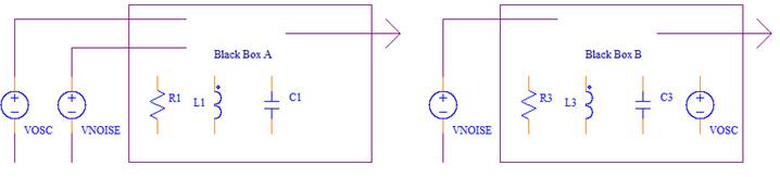
Black Box A is a linear, time invariant system, with external two inputs. Linear system theory states that such a system can only produce output frequencies contained by the two input sources.

Black Box B is physically the same system, but with VOSC hidden inside it. With respect to the now one external VNOISE signal, Black Box B is now a linear, time variant system. Black Box B can now, according to time variant system theory, produce frequencies not contained in its input signals. However, the system of VNOISE and Black Box B is still the same physical system, and so it still can not produce Δω MathType@MTEF@5@5@+=feaagCart1ev2aaatCvAUfeBSjuyZL2yd9gzLbvyNv2CaerbuLwBLnhiov2DGi1BTfMBaeXatLxBI9gBaerbd9wDYLwzYfdmGievaebbnrfifHhDYfgasaacH8YjY=vipgYlh9vqqj=hEeeu0xXdbba9frFj0=OqFfea0dXdd9vqai=hGuQ8kuc9pgc9q8qqaq=dir=f0=yqaiVgFr0xfr=xfr=xb9adbaqaaeGaciGaaiaabeqaamaabaabaaGcbaGaeuiLdqKaeqyYdChaaa@38E9@ mixed frequencies. Therefore, however calculated, Black Box B’s ISF zero order term c₀, must evaluate to zero. Thus the introduction of a linear LC system and its identification as a time variant system in an oscillator is not sufficient justification on its own that such a system can now magically produce up-converted mixed frequencies signals. The components themselves must change in time to produce such frequencies.

Yes 1/f Up Conversion

Consider the following oscillator:

Fig. 3

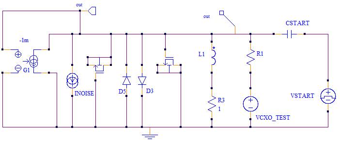
This oscillator is completely symmetrical, and produces a completely symmetrical oscillator waveform. Its ISF must therefore be completely symmetrical according to the HL-LTV theory, and hence have a zero value for its c_0,and subsequently, predict no up-converted phase noise. However, the Mosfets are non linear capacitors, being operated over their changing capacitance region. Low frequency noise appearing on those capacitors will therefore directly frequency modulate this oscillator and produce up-converted frequencies in contradiction the HL-LTV theory. As noted by A. Dimre, the resulting phase noise can be 50 dBc larger than that predicted by the HL theory, and as such, demonstrates that such a theory is, essentially useless for circuits of this nature, which, by and large is all of them.

Fully Symmetrical, Non-Linear Circuits Have Non Zero ISF

What is the real ISF of Fig. 3 ? That is, that function that, given an input signal, produces the output phase? For a non-linear capacitor system, the phase shifts produced by the same impulse on different corresponding points of a negative half cycle and a positive half cycle do not cancel because they will move the capacitance in different directions. A positive pulse on the positive half cycle will increase the magnitude of the voltage and hence increase the capacitance, where as on the negative half cycle that pulse will reduce the magnitude of the voltage and hence reduce the capacitance. Only if the capacitances remain constant, will the effect of the pulses cancel. Thus, the circuit of Fig. 3 will actually have a non-zero ISF in reality. The Linear part of the LTV is the nub of the problem. The ISF must be non-linear for non-linear capacitor circuits. HL- LTV engages much effort in trying to form a linear interpretation of phase noise generation, but this is inherently impossible, because the equations describing oscillators are inherently non linear differential equations.

Discussion

It is clear that the fundamental approach of the LTV method of calculating phase noise is seriously flawed. Real circuits are constructed from non-linear components, and these examples have shown that it is just not possible to accurately model many real, practical circuits by the LTV approach. It has been demonstrated that the real physics of an oscillator cannot be denied and hidden away in an abstract mathematical model. It may be argued then, that it is somewhat surprising that the HL-LTV theory is still be taught in universities. It is certainly a mystery to this author.

When is a theory wrong, and should be dispensed with, compared to when is a theory a usable approximation and retained?

The fact that a theory may sometimes, apparently give correct results does not imply that such a theory should retain any respect. For example, the Phlogiston theory of fire could, apparently, explain some aspects of fire, however, if an attempt was made to teach such a theory in a university, more than raised eyebrows would indeed be raised. In contrast, Newton’s Law Of Gravity, is a perfectly reasonable and accurate method of calculating all planetary motion for “low masses” and “low velocities” rather than using the far more complicated Einstein Field Equations.

Indeed, attention is drawn by way of example to what is often called “The Old Quantum Theory”. For example, the Bohr Model of the atom predicted quite well the atomic spectrum of Hydrogen, what with its quaint little electrons going in a circular orbit around a big fat proton. However, it is false, and professional physicists do not use it, but instead use standard Quantum Mechanics, for example, the Shrödinger Equation.

In the case of the LTV theory, it has been shown that the basic requirement of linearity is false for real circuits. It is also mathematically inconsistent. It may be said then that:

"The HL-LTV method can be shown to be valid for spherical chickens in a vacuum."

Website last modified 3^rd July 2013